Using the Chazelle, Kingsford, Singh Ampl Code

Download the Ampl code here.

Format of the input file

The input file should begin with the following line:

data;

Then specify the number of variable residues:

param num_posn := p ;

and the total number of rotamers:

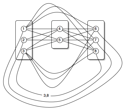
param num_nodes := n ;

Specify how many rotamers are in each position. The first column gives the position, the second gives the number of rotamers in that position. The sum of the position sizes must equal n.

param posn_size :=
   1 6
   2 81
   3 27
   ...
;

Specify the self-energies. Each rotamer is given a number between 1 and n. The rotamers of the first position are labeled 1 to the number of rotamers for the first residues. The rotamers in the second position are labeled with numbers starting right after the rotamers in the first position. The first column is the rotamer number, the second is the self-energy (in whatever units you want).

param costV :=
   1 3.254
   2 4.560
   3 6.721
   ...
;

Specify the pairwise energies. The first two columns are rotamer numbers involved in the interaction. The third column is the interaction energy (in whatever units you want). The number in the first column must be less than the number in the second column. Don't specify pairs that have zero energy between them.

param costE :=
   1 5 4.23
   1 6 -3.2
   3 5 -10
   ...
;

Optionally, specify the number of solutions you want. This option only has an effect for integer programs. It is ignored for linear programs.

param iterations := i ;

Comments may be specified anywhere in the file by starting a line with a "#" character. The comment extends to the end of the line. Whitespace and, except in comments, newlines are ignored so you can format the file in a way that is convenient.

An example input file: 1igd.native.dat.gz.

The entire dataset in this format is available here.

Solving the problem

Start Ampl (this is system dependent, usually by typing ampl). The following instructions show how to solve an LP. To solve an ILP, replace "cks_lp" with "cks_ilp" everywhere. At the ampl: prompt, load the model (what you would type is in italics):

ampl: model cks_lp.mod;

Load the particular problem you want to solve:

ampl: data 1igd.native.dat;

Then execute the Ampl script that matches the model you loaded:

ampl: commands cks_lp.ampl;

To save typing, the above process is wrapped into two simple scripts so you can say:

% solve_cks_lp 1igd.native.dat > 1igd.native.lpsol % solve_cks_ilp 1igd.native.dat > 1igd.native.lpsol

where "%" is your system's prompt. You should edit these scripts and change the value of the LP variable to point to the directory containing the .mod and .ampl files. Also, Ampl should be added to your PATH.

Format of the output file

The file will begin with some solver and version specific information in human-readable format, giving the problem size, solver options, times it took to run, etc.:

492002 variables, all linear
50064 constraints, all linear; 1032460 nonzeros
1 linear objective; 242837 nonzeros.

CPLEX 7.1.0: primal 
dualopt 
absmipgap=0
mipgap=1e-9
timing=1


Times (seconds):
  Input =  3.7 CPU 4.8 Wall
  Solve =  44 CPU 45 Wall
  Output = 0.36 CPU 0.43 Wall
CPLEX 7.1.0: optimal solution; objective -765.4709674
22929 dual simplex iterations (13037 in phase I)

The remaining sections of the file are delimited by lines beginning with "#" and a particular phrase. The order of the sections is fixed and the first one will be the energy of the optimal solution:

# energy
-765.4709673910816

The second section gives the problem dimensions: the first line gives the total number of rotamers; the second line gives the number of variables residues.

# problem size
1523
85

The next section gives the actual values for the node variables. If the solution is integral, it is these variables that specify which rotamer was chosen (1 = chosen, 0 = not chosen). The first column gives the rotamer number. The second indicates whether it was chosen. Lines for non-chosen rotamers may be omitted. For example:

# primal vertex variables
1 1
2 0
4 0
...

An example LP solution file: 1igd.native.lpsol.

Notes

By default, only the variables corresponding to nodes will be printed. Uncomment the section near the end of the .ampl files to also print the edge variables.
The .ampl files set the options for the CPLEX solver:
(LP) option cplex_options 'primal dualopt timing=1';
(ILP) option cplex_options 'primal dualopt absmipgap=0 mipgap=1e-9 timing=1';
We've found that primal dualopt is the fastest solver option. timing=1 prints how long CPLEX spent on the problem. absmipgap=0 mipgap=1e-9 are the strictest settings for the ILP. They force CPLEX to return the optimal solution, rather than some close approximation to it.
These options have been tested with CPLEX 7.1 and 7.5. Other versions may require slightly different options.
The Ampl code has been tested on Ampl version 20010215 on SunOS 5.7 and is known to parse with Ampl Student Version 20040229 on Linux.

visitors since July 27, 2004.
Last modified July 27, 2004.
Back to main page.