PVIEW: Princeton LC-MS/MS Data Viewer and Analyzer

This software implements the algorithms described in the following papers. Please cite these papers if you find PVIEW helpful for your work. Thanks!!!

• Zia Khan, Joshua S. Bloom, Benjamin A. Garcia, Mona Singh, and Leonid Kruglyak. Protein Quantification Across Hundreds of Experimental Conditions. Proceedings of the National Academy of Sciences. September 15, 2009 vol. 106 no. 37 15544-15548.
• Accurate proteome-wide protein quantification from high-resolution ¹⁵N mass spectra. Z. Khan(*), S. Amini(*), J. S. Bloom, C. Ruse, A. A. Caudy, L. Kruglyak, M. Singh, D. H. Perlman, and S. Tavazoie. Genome Biology 2011, 12:R122. (*) equal contribution. Supplemental data is available here.

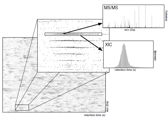
You can also read about the basic idea here:

• Space-partitioning speeds up data processing by Quinn Eastman. Journal of Proteome Research Online News. September 8, 2009

PVIEW has also been used successfully in the following papers:

• Impact of regulatory variation from RNA to protein, A. Battle(*), Z. Khan(*), S. H. Wang(*), A. Mitrano, M. J. Ford, J. K. Pritchard, Y. Gilad. Science 6 February 2015: Vol. 347 no. 6222 pp. 664-667. (*) equal contribution
• Stoichiometry of site-specific lysine acetylation in an entire proteome, J. Baeza, J. A. Dowell, M. J. Smallegan, J. Fan, D. Amador-Noguez, Z. Khan and J. M. Denu. August 1, 2014 The Journal of Biological Chemistry, 289, 21326-21338.
• Primate Transcript and Protein Expression Levels Evolve Under Compensatory Selection Pressures. Z. Khan, M. J. Ford, D. A. Cusanovich, A. Mitrano, J. K. Pritchard, Y. Gilad, Science. 29 November 2013: Vol. 342 no. 6162 pp. 1100-1104.
• Quantitative Measurement of Allele-Specific Protein Expression in a Diploid Yeast Hybrid by LC-MS. Z. Khan, J. Bloom, S. Amini, M. Singh, D. Perlman, A. Caudy, L. Kruglyak. Molecular Systems Biology (2012), 8:602. Supplemental data is available here.
• Global secretome analysis identifies novel mediators of bone metastasis. M. A. Blanco, A. LeRoy, Z. Khan, M. M. Aleckovic, B. M. Zee, B. A. Garcia, and Y. Kang. (2012) Cell Research (2012) 22:1339-1355. Highlight: Cell Research
• BclAF1 restriction factor is neutralized by proteasomal degradation and microRNA repression during human cytomegalovirus infection S. H. Lee, R. F. Kalejta, J. Kerry, O. J. Semmes, C. M. O'Connor, Z. Khan, B. A. Garcia, T. Shenk, and E. Murphy. Proceedings of the National Academy of Sciences, 109: 9575-9580, 2012.
• Direct targeting of Sec23a by miR-200s influences cancer cell secretome and promotes metastatic colonization M Korpal. F. M. Buffa, T. Ibrahim, M. A. Blanco, T. Celia-Terrassa, L. Mercatali, Z. Khan(*), H. Goodarzi, Y. Hua,Y. Wei, G. Hu, B. A. Garcia, J. Ragoussis, D. Amadori, A. L. Harris, Y. Kang. Nature Medicine 17, 1101-1108 (2011).

PVIEW has a number of useful features

• full GUI with cross platform support (Windows, MacOS, Linux)
• support for ETD fragmentation
• isotope labeled heavy vs. light quantification (e.g. SILAC)
• 15N heavy vs. light quantification
• isotope labeled heavy vs. medium vs. light (e.g. pulsed SILAC) quantification
• nonlinear alignment label-free quantification
• label free XIC-based quantification based on MS/MS DB search results
• XIC-based quantification where XICs are cross referenced based on their assigned peptide sequence
• integrated MS/MS database search
• internal reverse concatenated decoy database construction
• integrated FDR and q-value estimation using a reverse concanted decoy database
• support for external search engines (e.g. Mascot, SEQUEST, X! Tandem) via the PepXML file format
• protein grouping to account for isoforms and peptides that occur in many proteins
• completely open source
• support for data from Orbitrap, FTICR, and high resolution QTOF instruments
• tight integration with the R statistical programming language
• multi-threaded, PVIEW can take advantage of multiple CPU cores on your computer
• PVIEW is fast because it relies on space partitioning data structures

Sign up for the Google Groups email list by clicking here PVIEW Google Group.

System Requirements: For full data visualization capabilities, we recommend a computer with 8GB of RAM or more and a 64-bit operating system.

Source Code

You can now find the soruce code to pview on github at https://github.com/zia1138/pview.

PVIEW requires Qt version 5.0.x or newer and the Expat XML Parser version 2.0.1 or newer. The R Statistical Programming Language is highly recommended for data analysis.

Please read the included README for instructions on how to compile the source code for your operating system.

Binaries

• Windows 64-bit (17 July 2014)
• Windows 32-bit (23 December 2012) NOTE: The 32-bit version is not supported.

Column Descriptions

ratio.id

identifier of a specific XIC pair used for quantification

group.id

identifier associated with a particular group of proteins

protein.group

protein group, based on peptides identified, the most specific protein IDs possible

protein.group.nfrags

number of fragments within 6-40aa for each member of the protein group, useful for absolute quantification

group.N

number of ratios in each protein group

group.log2.HL.ratio

median heavy/light ratio for protein group

group.c

isotope pair condition, pulled from directory structure

group.r

isotope pair replicate, pulled from directory structure

group.i

isotope pair instrument run, pulled from file name

L.mz

m/z of light XIC in isotope pair

L.rt

retention time of light XIC in isotope pair

H.mz

m/z of heavy XIC in isotope pair

H.rt

retention time of heavy XIC in isotope pair

log2.HL.ratio

log2(heavy/light) ratio for pair pair

log2.xicH

area under of heavy XIC

log2.xicL

area under of light XIC

log2.xicHL.avg

average of area under XICs

ms2.scanNum

spectrum scan number for MS/MS ID

ms2.mz

precursor m/z for MS/MS spectrum

ms2.score

MS/MS search score

ms2.qvalue

q-value or FDR corrected significance for search result

ms2.charge

precursor charge of MS/MS spectrum

ms2.protein

proteins from which the search result can originate from, separated by ||||, use strsplit in R

ms2.protein.nfrags

number of fragments in 6-40aa range, useful for absolute quantification

ms2.seq

peptide sequences assigned to this isotope pair

ms2.missedcleaves

number of missed cleaves in peptide match

ms2.ppm.error

precursor mass error in PPMs

mz.theory

theoretical m/z for the peptide match

ms2.Nmods

number of variable modifications in peptide match

ms2.origin

XIC from which match was obtained (heavy or light)

ms2.shared

set to true if peptide is shared between multiple protein groups

Thermo2PVIEW: Converting .RAW files to PVIEW .mzXML

PVIEW takes only centroided mzXML files as input. For ThermoFisher LTQ-Orbitrap and LTQ-FTICR instruments, we recommend you collect the MS1 scans in profile mode and MS2 scans in centroid mode. If the data files are too big, centroid MS1 and centroid MS2 work just as well.

For your convenience, we provide a utility we call Thermo2PVIEW that will convert a directory of ThermoFisher LTQ-Orbitrap or LTQ-FTICR .RAW files into PVIEW compatible .mzXML files. Click here to download (Windows 64-bit, thermo2pview_win64_17jan2014.zip) the Windows binary.

In order to use Thermo2PVIEW you need to uncompress the .ZIP file and run MSFileReaderSetup.exe. Then try running the Thermo2PVIEW.EXE. If Thermo2PVIEW still doesn't run, try installing the Visual C++ redistributable package vcredist_x86.exe.

Thermo2PVIEW uses a library provided by ThermoFisher for accessing their .RAW files. MSFileReader. If you want to see the source code of Thermo2PVIEW, you can by clicking here to You can now find the soruce code to thermo2pview on github at https://github.com/zia1138/pview.

mzXML file organization

PVIEW can analyze complex experiments, but it requires you use a very specific directory structure for your files. First, you should create a directory with your experiment name (e.g. MyExperiment). In this folder, you should copy FASTA files containing the amino acid sequence information for your contaminant proteins, organismal proteins, and any other proteins you expect. These are merged into one single data base automatically. NOTE: No reverse/decoy databases are necessary PVIEW constructs them automatically!

For an isotope labeled experiment, lets say that you collect two experimental conditions relative to a common reference. For each of those two conditions you collected two replicates and for each replicate you used two gel or SCX fractions. You will have a total of 8 mzXML files from 8 instrument runs. These files should be organized as follows:

For alignment-based label-free quantification, the directory structure containing the mzXML files is a little different. lets say you ran 4 replicates of the same sample from condition #1 and four replicates of another sample from condition #2. Each of the 4 replicates can be divided into technical replicates consisting of two replicates each. For this experiment, you can organize the files as follows:

PVIEW will align the technical replicates first and then it will align the biological replicates. Last, it will align across conditions.

PepXML External Search Engine Support

PVIEW has an internal search engine, but also allows you to import search results from external search engines using the PepXML file format. In order to load PepXML files, create an additional directory under MyExperiment called pepxml.

In this directory put all of your validated PepXML files.

PVIEW will automatically detect PepXML files in this directory and load your search results.

You can convert the output of external search engines using tools from the TPP.

Keyboard Interface

• Z Press Z and draw box to zoom into data.
• X Zoom out.
• F Toggle filtered and raw peak data display.
• 1 Press 1 and draw box to select XICs (blue dots with lines) and display in dialog.
• 2 Press 2 and draw box to select XICs and display any contained MS/MS spectra in dialog.
• 3 Press 3 and draw box to select red MS/MS peaks.
• + Increase size of displayed peaks.
• - Decrease size of displayed peaks.
• R Cycle through range query region used for filtering and XIC construction
• G Display graph used to build XICs. Only works for filtered peak data.
• A Show region used for aligning to a reference instrument run or reference run set.
• P Display the retention time range used to group XICs across replicates.
• S Turn XIC display on and off. Also shows MS/MS IDs.
• I Display regions used to group XICs in stable-isotope mode or regions used to filter bad XICs in label-free mode
• O Display positions of grouped XICs across replicates and conditions

Algorithm Options and Parameters

Algorithm options and parameters are described below based organized by tab in the "Data Load Configuration" dialog box. The parameters descriptions are organized by tab. A lot of these parameters are in PPMs. Note that that ppm * 1e-6 * m/z = Da.

• number of CPU cores Number of CPUs to use to load and process the data.
• quantification mode isotope labeled or a label-free quantification modes
• keep raw peaks Keep raw peak data in memory.
• keep filtered peaks Keep filtered peaks.
• keep XIC peaks Keep chromatogram peaks (2d peaks).
• load MS/MS data Load MS/MS fragmentation spectra.
• keep MS/MS spectra After database search, keep MS/MS spectra in memory
• Run processing algorithms Run algorithms or just serve as a viewer.

• filter delta m/z (ppm) Height of orthogonal range/box query used to filter noise peaks in ppms.
• filter delta time Width of orthogonal range query used to filter noise peaks.
• peak threshold Minimum number of peaks returned in range queried to keep peak as signal.
• log10(I) histogram threshold log10(I) histogram threshold fraction
• XIC delta time Width of orthogonal range query used to construct XIC graph.
• XIC delta m/z (ppm) Height of orthogonal range query used to construct XIC graph.
• XIC min Minimum length in seconds of an XIC.
• XIC max Maximum length in seconds of an XIC.
• isotope tolerance Tolerance used for finding isotopic XICs (in PPMs).

• align translation Use retention time translation adjustment.
• align nonlinear Perform robust nonlinear alignment.
• align dtime Width in retention of query used to align.
• xic width m/z PPM width of box used to group across runs.
• group delta time Retention time window used for XIC grouping across runs.
• min conditions in group Minimum conditions a XIC must occur in.
• min replicate sets Minimum number of replicates represented by an XIC group (label-free only).
• min instrument runs Minimum number of runs represented by an XIC group (label-free only).
• skip median of median normalization Label free runs are normalized to adjust for differing protein amounts loaded.

• max label count Maximum number of labels per peptide (e.g. account for missed cleaves).
• *skip* normalize isotope ratios do not center the log2 ratio of each isotope pair around zero. Adjusts for loading error.
• use 15N metabolic labeling active 15N pairing
• Description a description for a custom user specified label
• Heavy mass shift A mass shift for a user specified label.
• Medium mass shift A medium mass shift for a user specified label (leave as zero by clocking OK in the shift calculator).
• Amion acids Amino acids that have the custom mass shift.
• Add/Remove Click to add and remove a custom isotope label

• precursor tolerance +- window in PPMs used for precursor mass
• MS2 tolerance +- window in (ppms or daltons) used for matching fragment peaks
• desired FDR False Discovery Rate (FDR) desired from database search. Estimate using a concatenated reverse decoy databse.
• missed cleavages Missed cuts by selected enzyme
• Lys-C, Trypsin, etc Enzyme used for theoretical digest
• max var modified AAs for variable modifications, this sets the limit on the number of amino acids that can be modified on a single fragment.
• desired site localization FDR maximum site FDR rate for PTM site localization

• Description description of the modification type
• Amino acids character codes of amino acids that are modified. List them with no spaces in between. Note that # specifies the protein N-terminus and * specified the protein C-terminus whereas [ and ] specify the cleavage N-terminus and C-terminus respectively.
• Mass shift Dalton shift in mass.
• use fixed 15N modifications database search on heavy 15N only labeled data

• Description descriptive name
• Abbreviation an abbreviation for the PTM used in spreadsheet output
• Mass mass shift of the precursor fragment
• Amino acids amino acids codes modified
• Frag. Mass shift shift relative to the precursor mass of the modification. This is usually zero except in the case of losses. To make this zero click the "..."
• Maximum count This parameter specifies the maximum number of times you can see this modification on a peptide. If it is 0, this implies it is only limited by the MS/MS search parameters
• +/- Add and remove a fragment modification mass shift.
• Add/Remove Add or remove a user-specified variable modification from the list

Tutorials

Stable Isotope labeled Quantification Tutorial

1. Download (VanHoof2009_subset.zip, 290MB) and unzip a subset of a large phosphoenriched data set. Note the original RAW files have already been converted to mzXML and centroided. The full data is from a the Cell Stem Cell paper Phosphorylation dynamics during early differentiation of human embryonic stem cells and can be download from Proteome Commons. It has the following Tranch hash number:
   g8hGaNTX/w5BHBEt9+NwoPQLeenbTK7xNKGFk23dkLpfEsf4IuHCLcXRBUjSwanxykWXwSjW51xGYRTzrLxKNGMkMugAAAAAAABsPg==
   
2. Make note of the directory structure. There are two time points and only one replicate of each time point in this subset.
3. Run PVIEW. Chose File > Open and select the VanHoof2009_subset directory that was created when you unzipped the data set.
4. Click through the tabs and make note of a few parameters. First, under the "Load" tab set the parameter "load threads" to the number of processors on your computer. Next, under the "Isotope" tab Lys8 and Arg10 are selected as labels. The "Use Isotope Mode" box is checked to indicate that isotope labeled quantification should be used. Under the "MS2" tab up to 4 variable mods are allowed per peptide and under the Variable tab each of STY phosphorylation is selected. Note also that under the "Memory" tab "Keep raw peaks" is unchecked. This is for systems that have smaller amount of RAM. If you have more than 4GB of RAM you should check "Keep raw peaks."
5. In order to load and process the data click the "Load data..." button. This will take a few minutes.
6. Once this processing is done you can navigate the data set using the keyboard commands. If you click on the "Isotope" tab, you will see a tree view of protein groups. Keep clicking until you see a tryptic fragment and for that fragment a list of ratios. You can double click on this ratio and entry and PVIEW will automatically jump to the corresponding isotope pair in the data set.
7. Next you can save and analyze the data by selecting the menu item "Isotope Pairs > Save All.." Find a destination directory and enter "VanHoof2009.txt" Once you do this PVIEW will generate several tab delimited table files VanHoof2009.txt (list of isotope pair ratios), VanHoof2009_corr.txt (data for correlating replicate isotope labeled runs, not really relevant here), VanHoof2009_internal.txt (data for computing protein level internal ratio correlations), VanHoof2009_internal_pep.txt (data for computing peptide level internal ratio correlations), VanHoof2009_mass_error_ms1.txt (precursor mass error data), VanHoof2009_mass_error_ms2.txt (MS/MS mass error using b1+ and y1+ fragment ions), VanHoof2009_table.txt (summary data in tabular format on a per-protein group basis), and VanHoof2009_table_pep.txt ( summary data in tabular format on a per-peptide basis).
8. With your version of PVIEW you should find an R Programming Language script called reports.R. Copy this into the directory containing all of the CSV files and run R in that directory. Run the following commands in R: source("reports.R") to load the script and isotope.pair.report("VanHoof2009.txt"). Run q() to quit R.
9. Running these R commands will create subdirectory called VanHoof2009 that will contain several useful plots. mass_error.pdf and mass_error2.pdf contain the precursor mass error and product ion mass error distributions respectively. internal_[30,240]min.pdf and internal_[30,240]min_Rep1.pdf correlates ratios of two groups of tryptic fragments from the same protein at the condition and replicate level. internal_[30,240]min_pep.pdf correlates duplicate measurements (e.g. different charge state) of the same peptide in the data. internal_[30,240]min_pep_mod.pdf does the same thing but for peptides with PTMs. For runs that have replicates of the same condition, you will also get plots that have the following name format: corr_xxxx.pdf. These correlate ratios across the replicates.
10. Any of the tab-delimited CSV files can be loaded into a spreadsheet program like Microsoft Excel. They can also be easily read into the R for statistical analysis by using the following command data <- read("VanHoof2009_xxx.txt", stringsAsFactors=F). You can run names("data") to get the column names in each CSV files.

Orbitrap Velos Data

1. Download (Velos.zip, 1.3GB) and unzip the data set. I've done the .mzXML conversion for you already
2. Run PVIEW. Chose File > Open and select the Velos directory that was created when you unzipped the data set.
3. In order to load and process the data click the "Load data..." button. This will take a few minutes.
4. Once this processing is done you can navigate the data set using the keyboard commands. If you click on the "Isotope" tab, you will see a tree view of protein groups. Keep clicking until you see a tryptic fragment and for that fragment a list of ratios. You can double click on this ratio and entry and PVIEW will automatically jump to the corresponding isotope pair in the data set.
5. Next you can save and analyze the data by selecting the menu item "Isotope Pairs > Save All.." Save the data by entering "Velos.txt" in the dialog box.
6. With your version of PVIEW you should find an R Programming Language script called reports.R. Copy this into the directory containing all of the CSV files and run R in that directory. Run the following commands in R: source("reports.R") to load the script and isotope.pair.report("Velos.txt"). Run q() to quit R. In the Velos sub-directory created by the R script, you should see several useful plots for assessing the data quality.

Alignment-Based Quantification Tutorial

1. Download (BYRMFoss2007.zip, 1.4GB) and unzip each of these 10 replicates each of yeast strains RM11-1a and BY4716 from the study Genetic basis of proteome variation in yeast by Foss et al.
2. Make note of the directory structure. Each of the FASTA files are the project BYRMFoss2007 directory. The ten replicates each of strain RM11-1a and BY4716 are in the RM and BY subdirectories respectively.
3. Run PVIEW. Chose "File > Open" and select the BYRMFoss207 directory. It was created when you unzipped the data set.
4. Click through the tabs and make note of a few parameters. First, under the "Load" tab set the parameter "load threads" to the number of processors on your computer. Click on the "Free" tab and notice that "Use align mode" is checked. This tells PVIEW to align LC-MS/MS runs. Also "align translation" and "align nonlinear" are checked to perform the maximum amount of retention time correction. Note that "min cond thres" is set to 2 requiring that a peptide should XIC occur in both strains and "Minimum instrument runs" is 5 designating that the signal occurs in 5 out of the 10 replicate instrument runs. Note also that under the "Memory" tab "Keep raw peaks" is unchecked. This is for systems that have smaller amount of RAM. If you have more than 4GB of RAM you should check "Keep raw peaks."
5. In order to load and process the data click the "Load data..." button. This will take a few minutes.
6. Once this processing is done you can navigate the data set using the keyboard commands. Try pressing the Z key and drawing a box. This will zoom into the data. Try hitting the S key to show the XICs with their IDs. Also try hitting the O key to show the aligned and grouped XICs across instrument runs. If you click on the "XIC" tab you will see a tree view of protein groups. Keep clicking until you see a tryptic fragment and for that fragment a list of area under the XIC values under the fragment. Double click on one of these and PVIEW will automatically jump to the corresponding XICs aligned in the data set.
7. Next, you can save and analyze the data by selecting the menu item "Label Free > Save CSV.." Find a destination directory and enter "BYRMFoss2007.txt" Once you do this PVIEW will generate several tab delimited table files BYRMFoss2007.txt ( per-protein quantification table), BYRMFoss2007_peptides.txt (per-peptide quantification table), BYRMFoss2007_internal.txt ( ratio correlations between all pairs of conditions), BYRMFoss2007_mass_error.txt ( precursor mass errors), and BYRMFoss2007_mass_error_ms2.txt (fragment ion mass errors).
8. With your version of PVIEW you should find an R Programming Language script called reports.R. Copy this into the directory containing all of the CSV files and run R in that directory. Run the following commands in R: source("reports.R") to load the script and internal.align.report("BYRMFoss2007.txt"). Run q() to quit R.
9. Running these R commands will create subdirectory called BYRMFoss2007 that will contain several useful plots. mass_error.pdf and mass_error2.pdf contain the precursor mass error and product ion mass error distributions respectively. interal_BY_RM.pdf computes ratios for each tryptic fragment between two conditions (here strains of yeast). If a protein has two or more tryptic fragments, it groups the fragment ratios into two groups and then correlates the two groups.
10. Any of the tab-delimited CSV files can be loaded into a spreadsheet program like Microsoft Excel. They can also be easily read into the R for statistical analysis by using the following command data <- read("BYRMFoss2007.txt", stringsAsFactors=F). You can run names("data") to get the column names in each CSV files.

XIC-based Quantification

License

Copyright (c) 2014, Princeton University, University of Maryland - College Park

All rights reserved.

Redistribution and use in source and binary forms, with or without modification, are permitted provided that the following conditions are met:

• Redistributions of source code must retain the above copyright notice, this list of conditions and the following disclaimer.
• Redistributions in binary form must reproduce the above copyright notice, this list of conditions and the following disclaimer in the documentation and/or other materials provided with the distribution.
• Neither the name of Princeton University or University of Maryland - College Park nor the names of its contributors may be used to endorse or promote products derived from this software without specific prior written permission.

THIS SOFTWARE IS PROVIDED BY THE COPYRIGHT HOLDERS AND CONTRIBUTORS "AS IS" AND ANY EXPRESS OR IMPLIED WARRANTIES, INCLUDING, BUT NOT LIMITED TO, THE IMPLIED WARRANTIES OF MERCHANTABILITY AND FITNESS FOR A PARTICULAR PURPOSE ARE DISCLAIMED. IN NO EVENT SHALL PRINCETON UNIVERSITY BE LIABLE FOR ANY DIRECT, INDIRECT, INCIDENTAL, SPECIAL, EXEMPLARY, OR CONSEQUENTIAL DAMAGES (INCLUDING, BUT NOT LIMITED TO, PROCUREMENT OF SUBSTITUTE GOODS OR SERVICES; LOSS OF USE, DATA, OR PROFITS; OR BUSINESS INTERRUPTION) HOWEVER CAUSED AND ON ANY THEORY OF LIABILITY, WHETHER IN CONTRACT, STRICT LIABILITY, OR TORT (INCLUDING NEGLIGENCE OR OTHERWISE) ARISING IN ANY WAY OUT OF THE USE OF THIS SOFTWARE, EVEN IF ADVISED OF THE POSSIBILITY OF SUCH DAMAGE.